Artificial Intelligence Virtual Experience Program - Cognizant
Table of Contents
Gala Groceries, a US-based tech-driven grocery chain, distinguishes itself through advanced technologies like IoT to gain a competitive advantage. Despite their commitment to offering top-notch, locally sourced fresh produce, maintaining consistent quality throughout the year poses challenges. Seeking Cognizant’s assistance, they aim to resolve a supply chain dilemma specific to perishable groceries, seeking to optimize stocking strategies and balance between excess storage costs and customer retention.
Objectives #
- Take a deep look at the problem by exploring the sample data provided thoroughly.
- Come up with a strategic plan to solve the problem, outlining the steps we need to follow.
- Perform feature engineering and develop a predictive model capable of forecasting the storage levels of each product.
- Make a pipeline for the Data Engineers to train the model on the provided dataset and make predictions along with evaluation.
Understanding the Problem #
Stock management, also known as inventory management, is a critical aspect of supply chain management that involves planning, organizing, and controlling the acquisition, storage, distribution, and utilization of goods. It encompasses various strategies and techniques aimed at maintaining an optimal balance between supply and demand while minimizing costs and ensuring efficient operations. Effective stock management is essential for businesses to meet customer demands, reduce carrying costs, and improve overall supply chain performance.
Importance of Stock Management in the Supply Chain:
- Meeting Customer Demand: Proper stock management ensures that products are available when and where customers want them. It prevents stockouts (running out of products) and overstock situations, allowing businesses to fulfill customer orders promptly and maintain high levels of customer satisfaction.
- Cost Control: Excess inventory ties up capital and incurs storage costs, while inadequate stock levels can lead to production disruptions and lost sales. Effective stock management helps strike a balance, reducing carrying costs, minimizing waste, and optimizing the use of resources.
- Supply Chain Efficiency: Efficient stock management contributes to the smooth functioning of the entire supply chain. By ensuring the right products are available at the right time, it minimizes disruptions and delays, leading to improved operational efficiency.
- Risk Mitigation: Fluctuations in demand, supply chain disruptions, and other external factors can impact a business’s ability to maintain steady stock levels. Effective stock management involves risk assessment and mitigation strategies to address potential disruptions and uncertainties.
- Working Capital Optimization: Excessive inventory ties up capital that could be invested in other areas of the business. Well-managed stock levels free up working capital, allowing companies to invest in growth opportunities or reduce debt.
- Supplier Relationships: Accurate stock management enables better communication with suppliers. Timely and accurate information about inventory levels helps in negotiating better terms, managing lead times, and building stronger relationships with suppliers.
Stock Management Techniques:
- Just-In-Time (JIT): JIT is a strategy where inventory is ordered and received only as needed for production or customer orders. It reduces carrying costs but requires precise coordination and reliable suppliers.
- Safety Stock: This involves maintaining a certain level of extra inventory to buffer against unexpected demand fluctuations or supply chain disruptions.
- ABC Analysis: Items are categorized into A, B, and C categories based on their value and contribution to sales. A-items (high-value) are closely monitored, while C-items (low-value) may have less stringent control.
- Economic Order Quantity (EOQ): EOQ calculates the optimal order quantity that minimizes the total cost of ordering and holding inventory. It considers factors like carrying costs, ordering costs, and demand.
- Cross-Functional Collaboration: Effective stock management involves collaboration between various departments like sales, marketing, production, and logistics to align inventory levels with overall business goals.
- Demand Forecasting: Accurate demand forecasting helps predict future demand patterns, enabling businesses to adjust stock levels accordingly.
- Technology and Automation: Inventory management software, barcoding, RFID, and IoT technologies can provide real-time visibility into stock levels and streamline stock tracking and replenishment processes.
In our case, we are combining IoT technologies that measures stock levels of different products with demand forecasting in order develop a model that can accurately predict the demand for each product and the best times to restock.
Data Exploration #
After assessing the quality of the data. We start our data exploration by visualizing the distribution of number of transactions per hour.
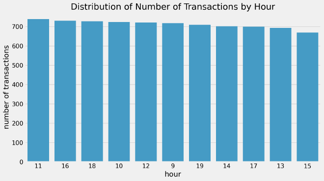
The number of transactions throughout the day are somewhat evenly distributed with 11am being the most active hour (738 transactions) and 3pm being the least active hour (669 transactions).
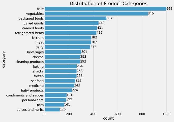
There are a few key takeaways from the above barplot, we mention:
- Fruits and Vegetables are the most sold categories making up 23.56% of the total transactions. This indicates a high demand for fresh products.
- packaged foods and baked goods also have a significant percentage of transactions, at 6.48% and 5.66% respectively.
- Canned foods, refrigerated items, and kitchen products have relatively lower percentages but still make up a noticeable portion of transactions.
- Meat, dairy, and beverages have similar percentages of around 4-5%, indicating that these categories are popular but are not purchased as much as fruits and vegetables.
- Cleaning products, baking supplies, snacks, and frozen items all have percentages in the range of 3-4%, indicating moderate demand for these categories.
- Seafood, medicine, baby products, condiments and sauces, personal care, pets, and spices and herbs have percentages below 3%, indicating a relatively lower demand for these categories.
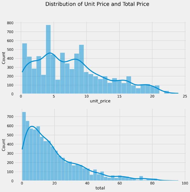
The first plot indicates that the distribution of unit price is positively skewed towards the lower end, implying that the majority of sales involve products with lower prices rather than higher ones.
This observation aligns with expectations for a typical grocery store, where a larger number of inexpensive products are sold compared to a smaller number of high-priced items.
Similarly, the second plot reveals a similar trend for the total price, indicating a positive skewness in its distribution. This implies that a larger proportion of sales transactions involve lower total prices compared to higher total prices.
Just as with unit prices, this observation is in line with the expectation that a grocery store would have a higher volume of transactions for lower-priced items, while fewer transactions would involve higher-priced items.
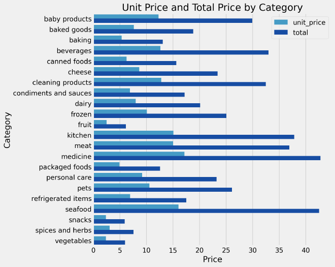
From the above figure representing the average unit prices and total prices for each category, here are the key takeaways:
- The unit prices and total prices vary across different categories, indicating differences in pricing for different types of products.
- Categories such as baby products, beverages, cleaning products, kitchen items, meat, medicine, and seafood have relatively higher unit prices and total prices. This suggests that these categories include higher-priced or premium products.
- Categories like fruit, snacks, spices and herbs, and vegetables have lower unit prices and total prices. This indicates that these categories consist of lower-priced or more affordable items.
- Categories like baked goods, dairy, frozen items, personal care, pets, and condiments and sauces have moderate unit prices and total prices, falling between the higher-priced and lower-priced categories.
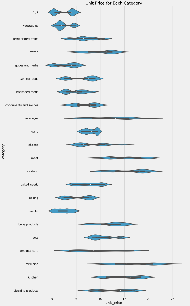
The analysis of the unit price distributions reveals an interesting pattern for several categories, namely fruit, vegetables, spices and herbs, canned foods, packaged foods, condiments and sauces, seafood, baking, kitchen, and cleaning products. These categories exhibit bimodal distributions, with two distinct peaks observed at different ends of the price spectrum.
This bimodality suggests the presence of two distinct qualities or tiers within these product categories. On one end of the spectrum, there are products with lower unit prices, indicating a more affordable or budget-friendly option. On the other end, there are products with higher unit prices, reflecting a premium or higher-quality offering.
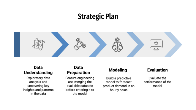
Strategic Plan #
Feature Engineering #
- Since we have three datasets –
sales,stock level, andtemperature– we should combine them using the datetime column. However, prior to merging, it’s necessary to round the time values to the nearest hour. - Merging datasets can create gaps due to missing values. Our solution involves judiciously applying suitable techniques to fill these gaps, ensuring a continuous and complete dataset. This process transforms missing values into valuable data points.
- While our dataset initially spans from 9am to 7pm, we recognize the need to encompass the entire day. By skillfully extending the dataset to cover all hours, we capture a broader context for analysis, thereby enriching the predictive capabilities.
- The dimension of time is unwrapped further, revealing three key temporal features:
hour,day, andmonth. These features introduce depth to the dataset, contributing to a more nuanced and accurate predictive model. - The path to accurate stock level prediction is illuminated by the Partial Autocorrelation Function (PACF) plot. Our analysis of this plot guides us to utilize lagged values of 1, 2, and 3, enabling the model to capture meaningful patterns and dependencies.
- Next we shifted other features -like
quantity,temperatureandtotalby one hour as it will be available at the time of making a prediction. customer_typeandcategorywere one hot encoded in order to be used for the model development.
Forecasting Model #
First, we split the data by using the first 6 days for training and 1 last day for testing.
train = data[data['ds']<'2022-03-07']
test = data[data['ds']>='2022-03-07']
train.drop('ds', axis=1, inplace=True)
test.drop('ds', axis=1, inplace=True)
Next, we seperate our target variable from the features that will be used to train the model.
y_train, y_test = train['y'], test['y']
X_train, X_test = train.drop('y', axis=1), test.drop('y', axis=1)
The following function will be used to evaluate the model performance. The evaluation metrics chosen are:
- Mean Squared Error: The average of the squared differences between predicted and actual values, used to measure the overall quality of a predictive model.
- Root Mean Squared Error: The square root of the average of the squared differences between predicted and actual values, providing a measure of the model’s prediction error in the same units as the original data.
- Mean Absolute Error: The average of the absolute differences between predicted and actual values, offering a straightforward measure of the model’s prediction accuracy.
- R Squared: A statistical measure indicating the proportion of the variance in the dependent variable that is explained by the independent variables in a regression model.
def evaluate(model_, X_test_, y_test_):
    y_pred = model_.predict(X_test_)

    results = pd.DataFrame({"MSE"  : [mean_squared_error(y_test_, y_pred)],
                            "RMSE" : [np.sqrt(mean_squared_error(y_test_, y_pred))],
                            "MAE"  : [mean_absolute_error(y_test_, y_pred)],
                            "R2"   : [r2_score(y_test_, y_pred)]})
    return results
Several machine learning and deep learning algorithms were implemented - namely:
- XGBRegressor
- LGBMRegressor
- Long Short Term Memory
GridSearchCV was used with XGBRegressor and LGBMRegressor for hyper parameter tuning.
XGBRegressor #
The XGBRegressor is a machine learning model belonging to the XGBoost (Extreme Gradient Boosting) framework: it is an ensemble learning technique designed for regression tasks, proficient at generating robust predictions. Within XGBoost, the XGBRegressor harnesses the collective power of multiple individual weak models to yield a potent predictive model. These weak models, in the context of XGBoost, are decision trees. The model employs a gradient boosting approach, wherein the algorithm iteratively constructs decision trees to minimize the discrepancies between predicted and actual target values.
Once the decision trees have been trained, XGBoost makes predictions by combining the predictions of all the trees using a weighted average. The weights for each tree are learned during training using the same objective function. This allows the algorithm to automatically learn which trees are more important and should be given more weight in the final prediction.
parameters = {'n_estimators':[128,200], 'max_depth':[7,9], 'learning_rate':[0.03,0.04]}
model = xgb.XGBRegressor(n_jobs=-1, random_state=44)
gs = GridSearchCV(model, parameters, scoring='neg_mean_squared_error', cv=5)
gs.fit(X_train, y_train)
The results shows that the best parameters for our model are summarized in the next table:
| Parameter | Value |
|---|---|
| learning_rate | 0.03 |
| max_depth | 7 |
| n_estimators | 128 |
The evaluation of the model gives the following results:
evaluate(gs, X_test, y_test)
| Metric | Score |
|---|---|
| Mean Squared Error | 226.496116 |
| Root Mean Squared Error | 15.049788 |
| Mean Absolute Error | 7.431851 |
| R Squared | 72.723% |
LGBMRegressor #
The LGBMRegressor, short for Light Gradient Boosting Machine Regressor, is a sophisticated machine learning model tailored for regression tasks. It falls under the domain of gradient boosting algorithms, specifically designed to provide rapid and highly accurate predictions. The distinguishing feature of the LGBMRegressor lies in its emphasis on optimization for efficiency and performance, making it particularly suitable for large datasets and complex regression problems.
Operating within the LightGBM framework, the LGBMRegressor leverages the power of ensemble learning, amalgamating the outputs of multiple weak models to formulate a robust collective prediction. The individual weak models in LightGBM are decision trees, which are constructed and refined through a gradient boosting process.
In each iteration, the LGBMRegressor constructs decision trees by learning from the residual errors of the preceding iterations, thereby enhancing its predictive capabilities iteratively. However, what sets LightGBM apart is its unique approach to constructing decision trees. It employs a histogram-based algorithm that optimizes the process of binning feature values, enabling faster and more efficient computation. This approach significantly reduces memory consumption and speeds up the training process, contributing to the model’s high efficiency and scalability.
parameters = {'n_estimators':[600,800], 'max_depth':[8,10], 'learning_rate':[0.04]}
model = LGBMRegressor(random_state=44)
gs = GridSearchCV(model, parameters, scoring='neg_mean_squared_error', cv=5)
gs.fit(X_train, y_train)
The results shows that the best parameters for our model are summarized in the next table:
| Parameter | Value |
|---|---|
| learning_rate | 0.04 |
| max_depth | 8 |
| n_estimators | 600 |
The evaluation of the model gives the following results:
evaluate(gs, X_test, y_test)
| Metric | Score |
|---|---|
| Mean Squared Error | 232.349011 |
| Root Mean Squared Error | 15.242999 |
| Mean Absolute Error | 6.929682 |
| R Squared | 72.0181% |
Long Short Term Memory #
Long Short-Term Memory (LSTM) is a type of recurrent neural network (RNN) architecture that has proven exceptionally effective in capturing and modeling sequential data, making it a cornerstone of modern machine learning and natural language processing tasks. Unlike traditional feedforward neural networks, LSTMs are explicitly designed to handle sequences by maintaining a memory of past information over extended time intervals, allowing them to comprehend patterns, dependencies, and context within sequential data.
The distinguishing feature of LSTMs is their ability to mitigate the vanishing gradient problem commonly encountered in standard RNNs. LSTMs achieve this by incorporating specialized gating mechanisms, including the input gate, forget gate, and output gate. These gates regulate the flow of information within the network, enabling it to retain relevant information over long periods while discarding or updating less relevant data.
The LSTM architecture consists of interconnected memory cells that can maintain their states over time, ensuring the network can capture and retain important patterns even across extended sequences. This makes LSTMs particularly well-suited for a wide range of applications, including time series forecasting, speech recognition, sentiment analysis, machine translation, and more. By preserving context and long-term dependencies, LSTMs have become a foundational tool in advancing the capabilities of deep learning models to process and comprehend sequential data with unparalleled accuracy and versatility.
For more information about LSTMs, I recommend the following youtube video
Since LSTMs do not support missing values, our initial task involves addressing this issue.
X_train.fillna(method='bfill', inplace=True)
X_train.fillna(method='ffill', inplace=True)
X_test.fillna(method='bfill', inplace=True)
X_test.fillna(method='ffill', inplace=True)
Next we will change the dimensions and data types before feeding the data to our network.
# Handle the dimensions
train_X = np.expand_dims(X_train.values, -1)
train_y = np.expand_dims(y_train.values, -1)
test_X = np.expand_dims(X_test.values, -1)
test_y = np.expand_dims(y_test.values, -1)
# Handle the data types
train_X = np.array(train_X, dtype=np.float32)
train_y = np.array(train_y, dtype=np.float32)
test_X = np.array(test_X, dtype=np.float32)
test_y = np.array(test_y, dtype=np.float32)
Finally, we build our model
model = Sequential()
model.add(LSTM(50, input_shape=(train_X.shape[1], train_X.shape[2])))
model.add(Dense(64, activation='relu'))
model.add(Dropout(0.2))
model.add(Dense(32, activation='relu'))
model.add(Dropout(0.2))
model.add(Dense(1))
model.compile(loss='mse', optimizer='adam')
# fit network
history = model.fit(train_X, train_y, epochs=50, batch_size=128, validation_data=(test_X, test_y), verbose=2, shuffle=False)
# plot history
plt.plot(history.history['loss'], label='train')
plt.plot(history.history['val_loss'], label='test')
plt.legend()
plt.show()
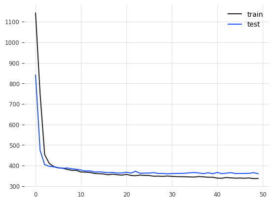
The evaluation of the model gives the following results:
evaluate(gs, X_test, y_test)
| Metric | Score |
|---|---|
| Mean Squared Error | 360.648804 |
| Root Mean Squared Error | 18.990755 |
| Mean Absolute Error | 11.528387 |
| R Squared | 56.5669% |
Key Findings #
- Model Performance and Validation: The top-performing model, LGBMRegressor, achieved MAE of 6.92, RMSE of 15.24, and an R2 score of 72.02%. Given the limited 7-day dataset (6 days for training, 1 day for testing), the model slightly underfits due to data scarcity.
Data scarcity refers to a situation where the available dataset is limited in size or lacks sufficient diversity. In the context of data science and machine learning, having a small amount of data can lead to challenges in building accurate and reliable models. When data is scarce, there might not be enough examples to capture the underlying patterns, relationships, and variations in the data. This can result in models that are less robust, less accurate, and more prone to overfitting or underfitting.
- Data Insights and Patterns: An intriguing discovery emerges from the data: distinct product categories exhibit a dual pricing structure, encompassing both budget-friendly and premium pricing tiers. What’s particularly interesting is that the budget-friendly range experiences higher purchase frequency, underscoring the market’s responsiveness to different pricing strategies.
- Lag Choice: We pick lags using a neat trick called partial autocorrelation. It helps the model choose the best past times for predicting the future. The model gets the time connections that make its predictions sharper.
- Assumptions and Limitations: An important consideration is the model’s temporal dependency on present data for hourly forecasts. Consequently, the model’s predictive horizon is constrained to a span of one hour. This limitation reflects the model’s reliance on immediate historical information to make short-term predictions.
Recommendations #
- Future Steps and Improvements: The path to a more robust forecasting model lies in the acquisition of a larger dataset. A greater volume of data would not only facilitate a deeper understanding of underlying seasonality but also enhance the precision of predictions. By capturing more intricate temporal patterns, the model’s accuracy could be substantially improved.
- Business Implications: A strategic recommendation involves the introduction of a new variable termed ‘restock’, which serves as an indicator of stock levels within the grocery shop. By setting a threshold—for instance, restocking when stock falls below 50%—the problem transforms into a classification task. Comparing the performance of this classification model with the one predicting stock levels can provide valuable insights into the approach used to solve the stock management problem for Gala Groceries.