Data Science & Analytics Virtual Experience Program - BCG
Table of Contents
PowerCo is a big company that provides gas and electricity to businesses, medium-sized enterprises, and homes. The energy market in Europe has changed, giving customers more options. This has caused many small and medium-sized businesses to switch to other energy providers, which is a big problem for PowerCo. To figure out why this is happening, they have teamed up with BCG for help.
Objectives #
- Gain a comprehensive understanding of the problem at hand and request necessary data from PowerCo to facilitate problem-solving.
- Conduct a thorough data exploration and examine the hypothesis that price sensitivity is somewhat associated with customer churn.
- Perform feature engineering and develop a predictive model capable of identifying customers with a high likelihood of churn.
- Prepare an executive summary summarizing the key findings and recommendations.
Understanding the Problem #
In business and marketing, churn refers to the rate at which customers or subscribers discontinue their relationship with a company or stop using its products or services. Therefore, the churn problem here refers to the challenge faced by powerCo in retaining its customers and reducing the rate of customer churn.
Understanding customer attrition (churn) is crucial for PowerCo as it allows them to identify patterns, trends, or factors that contribute to customer disengagement. The data needed to determine these patterns is:
- Billing data: Billing data can be used to determine how much customers are paying for their energy usage and how frequently they receive bills. This information can help to identify customers who are likely to be more price sensitive.
- Usage patterns: Information on customers’ energy usage patterns, such as the amount of energy they consume, the time of day they consume it, and their peak energy usage, may provide insights into their level of price sensitivity.
- Interaction history: like contract start date or whether there have been any concerns or complaints expressed by the customers. Any feature that would represent the customer’s satisfaction level.
- Churned: whether the customer enterprise churned or not.
Another useful data could be competitor’s information and their pricing so we can compare the costs relative to the competition in the field.
Data Exploration #
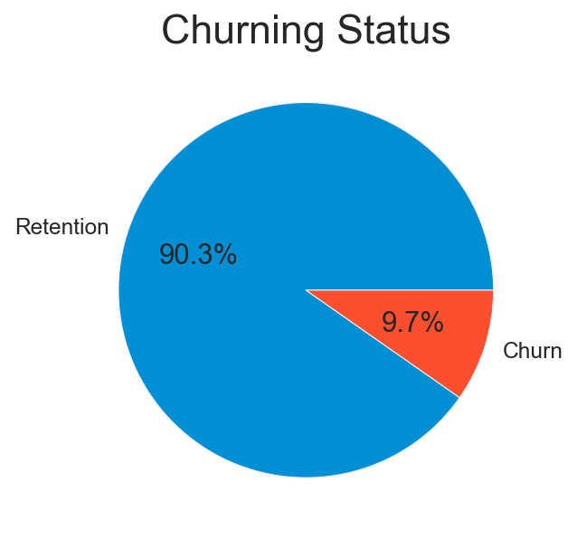
After assessing the quality of the data and cleaning it. We start our data exploration by visualizing the distribution of customers churn status.

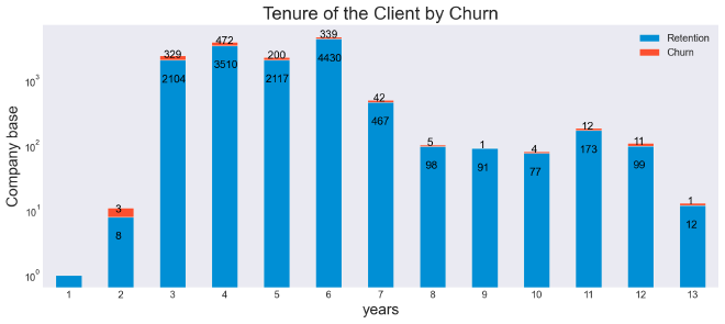
The majority of SME clients who churned have been with the company between 3 to 6 years. A concerning number of 28 SME have churned after being clients for PowerCo for more than 10 years as can be seen in the next barplot:

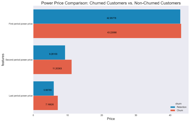
The next figure shows that churned SME pay more than those who did not churn. Which suggests that the pricing strategy is the reason of churn.

Hypothesis Testing: #
We will investigate further by hypothesis testing using two methods:
- Bootstrap.
- T-test.
We start by stating the null hypothesis and alternative hypothesis:
Null hypothesis: there is no significant difference between the mean of price of the two groups (churn/retention).
Alternative hypothesis: there is a significant difference between the mean of price of the two groups (churn/retention).
The significance level is assumed to be 5%.
Statistical significance is a term used in statistical hypothesis testing to describe the likelihood that an observed effect or difference between groups is real and not simply due to chance.
The p-values for both methods (Bootstrap/T-test) for the different price variables are less than the significance level leading to the rejection of the null hypothesis and suggesting that there is a difference between the mean of price of the two groups (churn/retention).
Feature Engineering #
Sum of price for energy and power along with the difference with respect to the period #
The changes in the price from one period to another is a good indicator for churn. The expected thing to notice is that SME who churned will have a positive difference meaning that the prices for energy and power are getting high. The inverse is expected for SME who did not churn.
# price for period 1
price_df['price_p1']=price_df['price_off_peak_var']+price_df['price_off_peak_fix']
# price for period 2
price_df['price_p2']=price_df['price_peak_var']+price_df['price_peak_fix']
# price for period 3
price_df['price_p3']=price_df['price_mid_peak_var']+price_df['price_mid_peak_fix']
# difference between the price for period 2 and period 1
price_df['pp12']=price_df['price_p2']-price_df['price_p1']
# difference between the price for period 3 and period 2
price_df['pp23']=price_df['price_p3']-price_df['price_p2']
# difference between the price for period 3 and period 1
price_df['pp13']=price_df['price_p3']-price_df['price_p1']
Difference between 1st period prices in December and preceding January #
This the prices progression in a different and more detailed way.
# Group off-peak prices by companies and month
monthly_price_by_id = price_df.groupby(['id', 'price_date']).agg({'price_off_peak_var': 'mean', 'price_off_peak_fix': 'mean'}).reset_index()

# Get january and december prices
jan_prices = monthly_price_by_id.groupby('id').first().reset_index()
dec_prices = monthly_price_by_id.groupby('id').last().reset_index()

# Calculate the difference
diff_1 = pd.merge(dec_prices.rename(columns={'price_off_peak_var': 'dec_1', 'price_off_peak_fix': 'dec_2'}), jan_prices.rename(columns={'price_off_peak_var': 'jan_1', 'price_off_peak_fix': 'jan_2'}).drop(columns='price_date'), on='id')
diff_1['diff_dec_january_energy_p1'] = diff_1['dec_1'] - diff_1['jan_1']
diff_1['diff_dec_january_power_p1'] = diff_1['dec_2'] - diff_1['jan_2']
diff_1 = diff_1[['id', 'diff_dec_january_energy_p1','diff_dec_january_power_p1']]
diff_1.head()
Difference between 2nd period/3rd period prices in December and preceding January #
These are calculated in the same way as the feature for the first period.
Tenure #
Tenure is a very important factor for predicting churn. it is the duration of business between the client and PowerCo.
df['tenure'] = (df['date_end']-df['date_activ']).dt.days/365
The deviation of last month consumption relative to the mean consumption for one month #
This feature aims at detecting any change of pattern in the consumption of the client for the last month.
df['cons_dev']=(df['cons_12m']/12)-df['cons_last_month']
Ratio of consumption for the next year compared to the current year #
This feature shows whether the client is expected to have a larger or lower demand for energy and power in the future compared to his current consumption.
df['cons_pattern']=df['forecast_cons_12m']/df['cons_12m']

def handleInf(x):
    if x==float('-inf') or x==float('inf'):
        return 0
    else:
        return x

# handle infinity values
df.cons_pattern=df.cons_pattern.apply(handleInf)
# handle a few missing values due to a division by 0
df['cons_pattern'].fillna(0, inplace=True)
Lastly, date features will dropped as they are summarized in a more representative feature that is tenure. And we drop any duplicates in the dataset to avoid having the same observations in the training and test sets.
train = pd.merge(price_df.drop(['price_date', 'price_off_peak_var', 'price_off_peak_fix', 'price_peak_var',
                                'price_peak_fix', 'price_mid_peak_var', 'price_mid_peak_fix'], axis=1),
                 df.drop(['date_activ', 'date_end', 'date_modif_prod', 'date_renewal'], axis=1), on='id')
# Drop duplicates
train.drop_duplicates(inplace=True)
Predictive Model Development #
First, we seperate our target variable from the features that will be used to train the model.
y = train['churn']
X = train.drop(['churn'], axis=1).set_index('id')
Then, we make some preprocessing to the data before giving it to the model.
# Convert has_gas column datatype to int
X['has_gas'] = X['has_gas'].astype(int)
# Encode channel_sales and origin features using a OneHotEncoder
ct = ColumnTransformer(transformers=[('encoder', OneHotEncoder(), [6,24])], remainder='passthrough')
X = np.array(ct.fit_transform(X))
We split the data into training and test sets of sizes 75% and 25% respectively. Making sure that the target variable is similarly distributed in both sets.
X_train, X_test, y_train, y_test = train_test_split(X, y, test_size=0.25, stratify=y)
The following function will be used to evaluate the model performance. The evaluation metrics chosen are:
- accuracy: however it is not representative for the model performance as predicting all 0’s will give an accuracy above 90%. This is why the next evaluation metrics are useed.
- Precision: it indicates how many of the predicted as
churnedare actually true. - recall: it explains how many of the actual positive cases we were able to detect with our model.
- f1 score: It gives a combined idea about Precision and Recall metrics. It is maximum when Precision is equal to Recall.
- ROC AUC: The Receiver Operator Characteristic (ROC) is a probability curve that plots the TPR(True Positive Rate) against the FPR(False Positive Rate) at various threshold values and separates the ‘signal’ from the ‘noise’. The Area Under the Curve (AUC) is the measure of the ability of a classifier to distinguish between classes.
def evaluate(model_, X_test_, y_test_):
    y_pred = model_.predict(X_test_)

    results = pd.DataFrame({"Accuracy"  : [accuracy_score(y_test_, y_pred)],
                            "Precision" : [precision_score(y_test_, y_pred)],
                            "Recall"    : [recall_score(y_test_, y_pred)],
                            "f1"        : [f1_score(y_test_, y_pred)],
                            "ROC AUC"   : [roc_auc_score(y_test, y_pred)]})
    return results
The model used is XGBClassifier: it is an ensemble learning method that combines the predictions of multiple weak models to produce a strong prediction. The weak models in XGBoost are decision trees, which are trained using gradient boosting. This means that at each iteration, the algorithm fits a decision tree to the residuals of the previous iteration.
Once the decision trees have been trained, XGBoost makes predictions by combining the predictions of all the trees using a weighted average. The weights for each tree are learned during training using the same objective function. This allows the algorithm to automatically learn which trees are more important and should be given more weight in the final prediction.
We used GridSearchCV for hyper parameter tuning.
parameters = {'n_estimators':[256,512,1024], 'max_depth':[6,8,12], 'learning_rate':[0.03,0.1]}
model = xgb.XGBClassifier(n_jobs=-1, random_state=44, use_label_encoder=False, eval_metric=f1_score)
gs = GridSearchCV(model, parameters, scoring='f1', cv=5)
gs.fit(X_train, y_train)
The results shows that the best parameters for our model are summarized in the next table:
| Parameter | Value |
|---|---|
| learning_rate | 0.1 |
| max_depth | 12 |
| n_estimators | 1024 |
The evaluation of the model gives the following very satisfying results:
evaluate(gs, X_test, y_test)
| Metric | Score |
|---|---|
| Accuracy | 0.997446 |
| Precision | 1.0 |
| Recall | 0.97397 |
| f1 Score | 0.986813 |
| ROC AUC | 0.986985 |
Recommendations #
The results obtained on the test set demonstrate outstanding performance in predicting customer churn. The precision metric indicates that all the clients identified as likely to churn did indeed churn, achieving a perfect 100% precision score. This high precision signifies the reliability of the predictive model in accurately identifying potential churners.
With such a reliable model in place, PowerCo can confidently implement targeted retention strategies for small and medium-sized enterprises (SMEs) who are predicted to be at high risk of churn. Offering a substantial 20% reduction in their energy costs can serve as a compelling incentive for these SMEs to remain loyal to PowerCo.
Implementing this personalized approach not only helps retain SME customers but also fosters a sense of loyalty and satisfaction among them. Additionally, it positions PowerCo as a proactive and customer-centric energy provider, capable of anticipating and addressing customer needs effectively.
It is important to note that while the model’s precision is exceptional, further considerations should be taken into account. Continuously monitoring and refining the predictive model will ensure its accuracy and effectiveness in identifying potential churners. Furthermore, evaluating the impact of the discount offer on customer retention and overall profitability will provide valuable insights for future decision-making and resource allocation.
Overall, the combination of an accurate predictive model and a targeted discount strategy presents an opportunity for PowerCo to reduce churn rates, enhance customer loyalty, and maintain a competitive edge in the energy market.
Executive Summary #
