Building an End-to-End MLOps Pipeline for Air Quality Forecasting 🌍

Air quality forecasting is crucial for public health, yet building a production-ready system that continuously learns and adapts requires more than just a good model—it demands a robust MLOps infrastructure. This project represents my journey into building an end-to-end MLOps pipeline that forecasts the European Air Quality Index (AQI) for 13 regions in France, predicting up to 12 hours ahead. Through this experience, I learned that successful ML systems are built on three pillars: reliable data pipelines, thoughtful feature engineering, and seamless deployment infrastructure.

The system I built collects real-time data from the Open-Meteo Air Quality API, stores it in Hopsworks feature stores, trains XGBoost models for multi-horizon forecasting, and serves predictions through an automated pipeline. What makes this project particularly valuable is not just the forecasting accuracy, but the complete MLOps ecosystem that ensures the system remains reliable, scalable, and maintainable in production.

This blog shares the key learnings, technical challenges, and architectural decisions that went into building this system. From understanding temporal patterns through autocorrelation analysis to implementing automated pipelines with GitHub Actions, each component taught me something new about building production ML systems.

The Challenge: From Data to Predictions #

Forecasting air quality is inherently a time series problem with unique characteristics:

• Multi-horizon predictions: We need forecasts for 1h, 2h, up to 12h ahead, not just a single point
• Multi-region forecasting: 13 different regions, each with distinct patterns
• Real-time updates: The system must adapt to new data continuously
• Production reliability: The pipeline must run automatically without manual intervention

These requirements pushed me to design a system that goes beyond a simple Jupyter notebook. I needed versioned data storage, automated model training, reliable serving infrastructure, and monitoring capabilities—the hallmarks of a proper MLOps pipeline.

Data Collection: Building a Reliable API Pipeline #

The foundation of any ML system is quality data. For this project, I leveraged the Open-Meteo Air Quality API, which provides European AQI data based on CAMS (Copernicus Atmosphere Monitoring Service) forecasts. The API offers hourly data at approximately 11km spatial resolution, covering all 13 French regions.

API Integration Challenges #

One of the first lessons I learned was that API reliability is non-negotiable. Initial implementations failed silently when the API was temporarily unavailable, leading to data gaps that propagated through the entire pipeline. Here’s how I built resilience:

# Setup the Open-Meteo API client with cache and retry on error
cache_session = requests_cache.CachedSession('.cache', expire_after=-1)
retry_session = retry(cache_session, retries=5, backoff_factor=0.2)
openmeteo = openmeteo_requests.Client(session=retry_session)

The key improvements included:

• Request caching: Using requests-cache to avoid redundant API calls during development
• Exponential backoff: Implementing retry logic with retry-requests to handle transient failures
• Batch requests: Fetching data for all 13 regions in a single API call to minimize latency

Efficient Data Storage #

Rather than storing raw API responses, I designed a data ingestion pipeline that:

1. Fetches only new data (incremental updates)
2. Validates data completeness before storage
3. Stores data in Hopsworks feature groups for versioning and lineage

def fetch_data(aqi_fg, aqi_df, regions_df, last_dates, start_hour, end_hour):
    # Get last 24 hours from existing data
    last_24h = aqi_df[aqi_df['date'] >= aqi_df['date'].max() - pd.Timedelta(hours=24)].copy()
    
    # Fetch new data from API
    retrieved_df = fetch_from_api(regions_df, start_hour, end_hour)
    
    # Filter out existing data to avoid duplicates
    filtered_df = retrieved_df.merge(last_dates, on="region_id", how="left")
    filtered_df = filtered_df[filtered_df["date"] > filtered_df["last_date"]]
    
    # Insert only new records
    aqi_fg.insert(filtered_df)

This incremental approach ensures we never duplicate data while maintaining a complete historical record. The feature group in Hopsworks automatically handles versioning, allowing us to track changes over time and roll back if needed.

Feature Engineering: Understanding Temporal Patterns #

Time series forecasting requires understanding the temporal dependencies in the data. Simply using the current AQI value isn’t sufficient—we need to capture patterns like daily cycles, recent trends, and seasonal variations.

Autocorrelation Analysis: Finding the Right Lags #

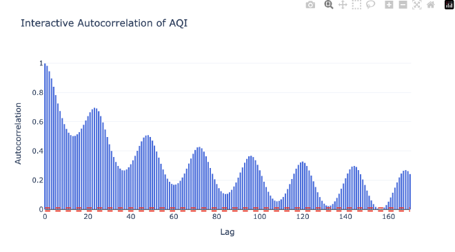
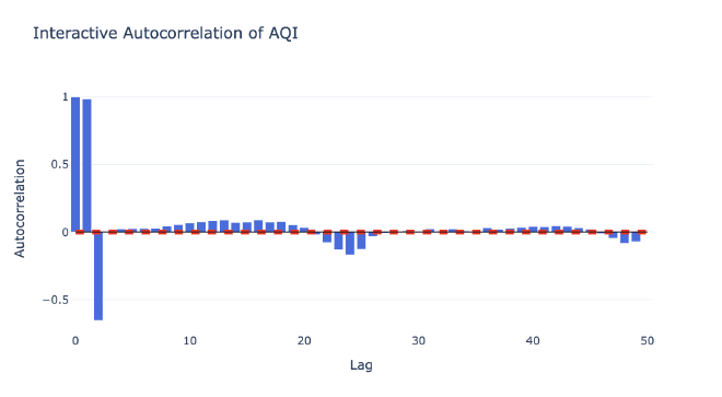
The most critical step in feature engineering was identifying which historical time points are most predictive of future AQI values. This is where autocorrelation analysis came in. I used ACF (Autocorrelation Function) and PACF (Partial Autocorrelation Function) plots to understand the temporal structure of the data.

Key Insights from Autocorrelation Analysis #

The ACF and PACF plots revealed several important patterns:

1. Short-term dependencies (lags 1-6): Strong correlations indicating that recent AQI values are highly predictive of near-future values. This makes intuitive sense—air quality changes gradually, not abruptly.

2. Daily cycle (lags 23-25): Significant correlations at ~24 hours, reflecting daily patterns in air quality. This captures effects like traffic patterns, industrial activity cycles, and weather patterns that repeat daily.

3. Weekly patterns: While not as strong as daily patterns, there were subtle weekly cycles that could be valuable for longer-horizon forecasts.

Based on this analysis, I selected lags [1, 2, 3, 4, 5, 6, 23, 24, 25] as features. This combination captures both immediate trends and daily cycles without overcomplicating the model.

Creating Lag Features #

The feature engineering pipeline transforms raw AQI values into a rich feature set:

def create_features_and_targets(feature_view, config):
    df_region = feature_view.get_batch_data()
    df_region = df_region.sort_values('date').reset_index(drop=True)
    
    # Create lag features
    for lag in config['input_lags']:
        df_region[f'lag_{lag}'] = df_region['european_aqi'].shift(lag)
    
    # Create target features (forecast horizon)
    for step in range(1, config['forecast_horizon'] + 1):
        df_region[f'target_t_plus_{step}'] = df_region['european_aqi'].shift(-step)
    
    # Drop rows with NaN values (due to shifting)
    df_training = df_region.dropna().reset_index(drop=True)
    
    return df_training

This approach creates:

• 10 input features: Current AQI + 9 lag features (lags 1, 2, 3, 4, 5, 6, 23, 24, 25)
• 12 target variables: Forecasts for +1h through +12h

The shift operation creates the temporal features while the negative shift creates future targets for training. This is a standard approach in time series forecasting, but getting the lag selection right was crucial for model performance.

Model Training: Multi-Output Forecasting with XGBoost #

Forecasting 12 horizons simultaneously requires a model that can learn complex relationships between input features and multiple outputs. I chose XGBoost wrapped in a Multi-Output Regressor for several reasons:

1. Handles non-linear relationships: Air quality patterns aren’t linear—XGBoost captures complex interactions
2. Feature importance: Provides interpretability into which lags matter most
3. Robust to outliers: Air quality data can have spikes due to events
4. Efficient training: Fast training even with large datasets

Model Architecture #

def train_model(X_train, Y_train):
    # Initialize XGBoost base regressor
    base_model = xgb.XGBRegressor(
        objective='reg:squarederror',
        n_estimators=500,
        learning_rate=0.05,
        max_depth=6,
        subsample=0.8,
        colsample_bytree=0.8,
        reg_alpha=0.1,      # L1 regularization
        reg_lambda=1.0,     # L2 regularization
        random_state=42,
    )
    
    # Wrap it for multi-step output
    model = MultiOutputRegressor(base_model, n_jobs=-1)
    
    # Fit model
    model.fit(X_train, Y_train)
    
    return model

The MultiOutputRegressor wrapper trains separate XGBoost models for each forecast horizon. This approach allows each horizon to have its own optimized model while sharing the same feature set. In practice, this means the model learns different patterns for short-term (1-3h) versus longer-term (10-12h) forecasts.

Training Strategy #

A critical decision was how to split the data for training and testing. I used a time-based split, keeping the most recent 6 months as the test set:

# Find the last date in the dataset
last_date = df_region['date'].max()

# Calculate cutoff date (6 months before last date)
cutoff_date = last_date - pd.DateOffset(months=config['months_before_last'])

df_training = df_region[df_region['date'] <= cutoff_date].dropna()
df_test = df_region[df_region['date'] > cutoff_date].dropna()

This temporal split ensures the model is evaluated on data it hasn’t seen during training, simulating real-world performance. The 6-month cutoff provides enough test data to evaluate performance across different seasons and conditions.

Evaluation Metrics #

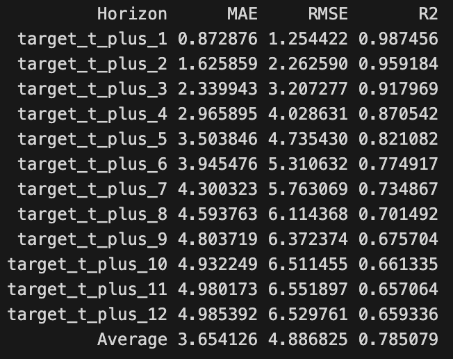
For multi-horizon forecasting, I track performance at each horizon separately:

def evaluate_forecasts(Y_test, Y_pred):
    metrics = []
    for i, horizon in enumerate(range(1, 13)):
        y_true = Y_test.iloc[:, i]
        y_hat = Y_pred[:, i]
        
        mae = mean_absolute_error(y_true, y_hat)
        rmse = np.sqrt(mean_squared_error(y_true, y_hat))
        r2 = r2_score(y_true, y_hat)
        
        metrics.append({
            "Horizon": f"+{horizon}h",
            "MAE": mae,
            "RMSE": rmse,
            "R2": r2
        })
    
    return pd.DataFrame(metrics)

This granular evaluation revealed that short-term forecasts (1-3h) are significantly more accurate than longer-term forecasts (10-12h), which is expected as uncertainty increases with forecast horizon.

MLOps with Hopsworks: Production-Ready Infrastructure #

Building a model is only half the battle—deploying it reliably in production requires proper MLOps infrastructure. This is where Hopsworks became invaluable, providing feature stores, model registry, and model serving in a unified platform.

Feature Store: Versioned Data Management #

Hopsworks feature stores solve several critical problems:

• Data versioning: Track how data changes over time
• Feature reuse: Share features across multiple models
• Online/offline storage: Support both batch training and real-time serving

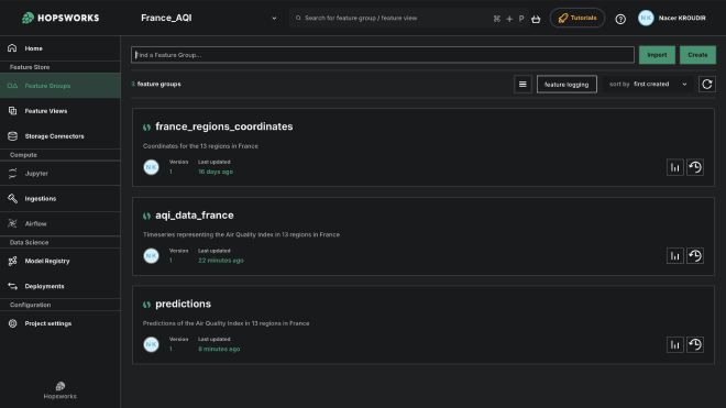
I created three main feature groups:

1. france_regions_coordinates: Static region metadata (coordinates, names)
2. aqi_data_france: Historical AQI observations with primary key (region_id, date)
3. predictions: Model predictions for all 13 regions and 12 horizons

# Create feature group
aqi_fg = fs.get_or_create_feature_group(
    name='aqi_data_france',
    version=1,
    primary_key=['region_id', 'date'],
    description='European AQI data for French regions'
)

# Create feature view for training
feature_view = fs.get_or_create_feature_view(
    name="aqi_forecast",
    version=1,
    query=aqi_fg.select(['region_id', 'date', 'european_aqi']),
)

The feature view abstracts the underlying data sources, making it easy to change data sources without modifying training code. This separation of concerns is a key MLOps best practice.

Model Registry: Versioned Model Management #

The model registry tracks model versions, metrics, and metadata:

# Convert metrics to dictionary format
metrics_dict = {}
for record in test_results.to_dict(orient="records"):
    horizon = record['Horizon']
    for metric_name in ['MAE', 'RMSE', 'R2']:
        key = f"{horizon}_{metric_name}"
        metrics_dict[key] = record[metric_name]

# Register model in Hopsworks
py_model = mr.python.create_model(
    "xgboost",
    metrics=metrics_dict,
    feature_view=feature_view
)
py_model.save("models/model.joblib")

This registration captures:

• Model artifacts (the trained model file)
• Performance metrics for each horizon
• Link to the feature view used for training
• Training metadata (timestamps, configurations)

Having this registry allows me to compare model versions, roll back to previous models if performance degrades, and understand which features and data were used for each model.

Model Serving: Automated Predictions #

The most impressive part of the Hopsworks platform is model serving. Instead of manually loading models and making predictions, Hopsworks provides a deployment system that handles scaling, monitoring, and reliability:

def start_deployment(project):
    ms = project.get_model_serving()
    mr = project.get_model_registry()
    
    # Get the model from registry
    model = mr.get_model("xgboost", version=1)
    
    # Create predictor with script file
    predictor = ms.create_predictor(model, script_file="src/predictor_file.py")
    
    # Create deployment
    deployment = ms.create_deployment(predictor, name="xgboost")
    deployment.start(await_running=300)
    
    return deployment

The predictor script defines how to load the model and make predictions:

class Predict(object):
    def __init__(self, async_logger, model):
        project = hopsworks.login()
        self.mr = project.get_model_registry()
        
        # Load the trained model
        self.model = joblib.load(os.environ["MODEL_FILES_PATH"] + "/model.joblib")
    
    def predict(self, data):
        prediction = self.model.predict(data).tolist()
        return prediction

This deployment system automatically:

• Scales based on demand
• Monitors prediction latency and errors
• Provides REST API endpoints for predictions
• Handles model updates without downtime

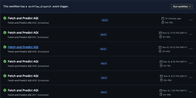
Automated Pipeline: GitHub Actions #

To make the system truly production-ready, I automated the entire pipeline using GitHub Actions. The workflow runs every hour, fetching new data and generating predictions:

name: Fetch and Predict AQI

on:
  schedule:
    # Run at 2 minutes past every hour
    - cron: '2 * * * *'
  workflow_dispatch: # Allows manual triggering

jobs:
  fetch-and-predict:
    runs-on: ubuntu-latest
    steps:
    - name: Checkout repository
      uses: actions/checkout@v4
    
    - name: Set up Python
      uses: actions/setup-python@v5
      with:
        python-version: '3.12.4'
    
    - name: Install dependencies
      run: pip install -r requirements.txt
    
    - name: Run fetch and predict script
      env:
        HOPSWORKS_API_KEY: ${{ secrets.HOPSWORKS_API_KEY }}
      run: python src/fetch_and_predict.py

This automation ensures:

• Continuous updates: New data is fetched hourly without manual intervention
• Automatic predictions: Forecasts are generated and stored immediately after data updates
• Error handling: The workflow includes retry logic and logging for debugging
• Reproducibility: Every run is logged and can be reproduced

The pipeline follows this flow:

1. Fetch latest AQI data from Open-Meteo API
2. Store new data in Hopsworks feature store
3. Prepare features with lag variables
4. Load model from registry and start deployment
5. Generate predictions for all regions
6. Store predictions in feature store
7. Stop deployment to save resources

Interactive Dashboard: Real-Time Visualization #

A model is only useful if users can interact with it. I built a comprehensive Streamlit dashboard that provides real-time visualization of forecasts, model performance, and regional insights.

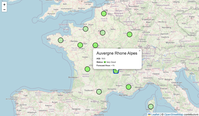
Overview Dashboard: Interactive France Map #

The dashboard’s centerpiece is an interactive map of France showing color-coded AQI forecasts:

def _create_france_map(regions_df, aqi_values, selected_hour):
    # Initialize map centered on France
    m = folium.Map(location=[46.5, 2.0], zoom_start=6)
    
    # Add markers for each region
    for _, row in regions_df.iterrows():
        region_id = row['region_id']
        aqi = aqi_values.get(region_id, np.nan)
        color = get_aqi_color(aqi)
        
        folium.CircleMarker(
            location=[row['latitude'], row['longitude']],
            radius=15,
            popup=f"{row['region']}: AQI {aqi:.1f}",
            color=color,
            fill=True,
            fillColor=color,
        ).add_to(m)
    
    return m

Users can:

• Select forecast horizon: Slider to view forecasts from +0h to +12h
• Click regions: See detailed information for each region
• View color coding: Green (good) to red (poor) based on AQI levels

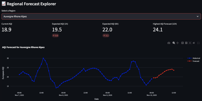
Regional Forecast Explorer #

For detailed analysis, users can select a specific region to view:

• Historical AQI: Last 72 hours of observed AQI values
• 12-hour forecast: Line chart showing predicted AQI for the next 12 hours
• Key metrics: Current AQI, expected change, maximum forecasted AQI

def render_regional_forecast(aqi_df, regions_df, predictions_df, latest_pred_date):
    # Get historical AQI (last 72 hours)
    historical = aqi_df[aqi_df['region_id'] == selected_region_id]
    historical = historical[historical['date'] >= historical['date'].max() - pd.Timedelta(hours=72)]
    
    # Get predictions
    forecast_values = []
    for h in range(1, 13):
        forecast_values.append(preds.iloc[0][f'target_t_plus_{h}'])
    
    # Create combined chart
    fig = go.Figure()
    fig.add_trace(go.Scatter(x=historical['date'], y=historical['european_aqi'], name='Historical'))
    fig.add_trace(go.Scatter(x=forecast_dates, y=forecast_values, name='Forecast'))
    
    st.plotly_chart(fig, use_container_width=True)

This visualization helps users understand:

• Trends: Is air quality improving or worsening?
• Forecast uncertainty: How do predictions compare to recent observations?
• Regional differences: Which regions have better or worse air quality?

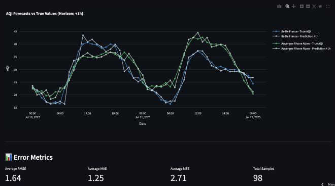
Evaluation & Insights: Model Performance Analysis #

The dashboard includes a comprehensive evaluation panel for analyzing model performance:

• Interactive evaluation: Select prediction horizon, date range, and regions
• Forecasts vs Actuals: Side-by-side comparison of predictions and observed values
• Performance metrics: MAE, RMSE, and R² scores by region and horizon
• Error heatmap: Visual representation of errors across regions and horizons
• Performance trends: How model performance changes over time

def calculate_metrics_for_evaluation(actual_df, pred_df, horizon, date_range=None):
    # Merge actual and predicted values
    merged = actual_df.merge(pred_df, on=['region_id', 'date'], how='inner')
    
    # Extract predictions for selected horizon
    pred_col = f'target_t_plus_{horizon}'
    y_true = merged['european_aqi']
    y_pred = merged[pred_col]
    
    # Calculate metrics
    mae = mean_absolute_error(y_true, y_pred)
    rmse = np.sqrt(mean_squared_error(y_true, y_pred))
    r2 = r2_score(y_true, y_pred)
    
    return {'MAE': mae, 'RMSE': rmse, 'R2': r2}

This evaluation capability is crucial for:

• Model monitoring: Detecting performance degradation over time
• Regional analysis: Understanding which regions are harder to forecast
• Horizon analysis: Seeing how forecast accuracy changes with horizon
• Data quality: Identifying regions or time periods with data issues

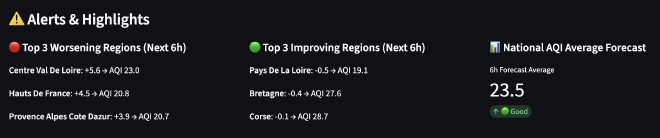
Alerts & Highlights #

To help users quickly identify important changes, the dashboard includes an alerts section:

• Top 3 worsening regions: Regions expected to have the largest AQI increases in the next 6 hours
• Top 3 improving regions: Regions expected to see the largest AQI decreases
• National average: Overall AQI trend across all regions

This feature transforms raw predictions into actionable insights, helping users prioritize which regions need attention.

Key Learnings and Challenges #

Building this end-to-end MLOps pipeline taught me several valuable lessons:

1. Data Quality is Paramount #

The biggest challenge wasn’t building the model—it was ensuring data quality. Missing data, API failures, and data format changes can break the entire pipeline. Building robust error handling, data validation, and incremental update logic was crucial.

2. Feature Engineering Matters More Than Model Complexity #

Spending time on autocorrelation analysis and selecting the right lags had a bigger impact on performance than tuning hyperparameters. Understanding the temporal structure of the data is essential for time series forecasting.

3. MLOps Infrastructure Enables Iteration #

Having proper MLOps infrastructure (feature stores, model registry, automated pipelines) made it easy to experiment, compare model versions, and deploy updates. Without this infrastructure, each iteration would have been manual and error-prone.

4. Visualization Drives Understanding #

The dashboard wasn’t just a nice-to-have—it was essential for understanding model behavior, identifying issues, and communicating results to stakeholders. Interactive visualizations revealed patterns that weren’t obvious from metrics alone.

5. Automation Reduces Technical Debt #

Automating the pipeline with GitHub Actions eliminated manual work and reduced the chance of errors. The hourly automated runs ensure the system stays up-to-date without requiring constant attention.

Future Improvements #

While the current system is production-ready, several enhancements could improve it further:

Model Improvements #

• Ensemble methods: Combining multiple models (XGBoost, LSTM, Prophet) could improve accuracy
• External features: Incorporating weather data, traffic patterns, or industrial activity could enhance predictions
• Uncertainty quantification: Providing prediction intervals, not just point forecasts

Infrastructure Improvements #

• Model monitoring: Automated alerts when model performance degrades
• A/B testing: Comparing model versions in production
• Feature store enhancements: Online feature serving for real-time predictions

Dashboard Enhancements #

• Alert system: Email or SMS notifications for poor air quality forecasts
• Historical analysis: Long-term trends and seasonal patterns
• Comparative analysis: Compare forecasts across different models or time periods

Conclusion #

Building this MLOps pipeline for air quality forecasting was a comprehensive learning experience that spanned data engineering, machine learning, and software engineering. The system demonstrates how modern MLOps tools can transform a research project into a production-ready application.

The key takeaway is that successful ML systems require more than just a good model—they need reliable data pipelines, thoughtful feature engineering, robust deployment infrastructure, and user-friendly interfaces. By combining these components, we can build systems that not only make accurate predictions but also remain maintainable, scalable, and useful in production.

The Hopsworks platform was particularly valuable, providing feature stores, model registry, and model serving in a unified system. This eliminated the need to build these components from scratch and allowed me to focus on the core ML challenges.

For anyone building similar systems, my advice is to invest in MLOps infrastructure early. The time spent setting up feature stores, model registries, and automated pipelines pays dividends as the system grows and evolves. The infrastructure enables rapid iteration, reliable deployment, and continuous improvement—the hallmarks of a successful ML system.